Solving a Wooden Puzzle Using Haskell (Part I)

April 28, 2025

This post is the first of a two-part series that describes my computer-assisted solution to a physical puzzle I got. In this first part, I describe the problem and model it in Haskell. This post is a little verbose, so feel free to skip directly to part II, where we'll see how to tell our computer to actually solve the puzzle.

I got gifted a puzzle recently, allegedly a "very hard one". After receiving it, I spent a couple minutes trying to solve it, but it quickly became clear that, unless there was a trick I'd missed, I didn't have the right combination of patience and brainpower for that. I had some family and friends try to solve it too, and although some of them displayed an impressive amount of persistence, none was persistent enough to crack the puzzle either.

You know who else is incredibly persistent? My computer. It's not nearly as smart as the humans around me and I, but it makes up for that in speed and tirelessness. So if I manage to tell it exactly what to do, it might be able to find a solution. Let's try!

The source for this post and the next is a literate Haskell file. This means you can run the code by running cabal run wooden_puzzle.lhs. You can also experiment with the values defined in it by running cabal repl wooden_puzzle.lhs.

The following pieces of code are here to tell the Haskell toolchain how exactly to interpret the file, and what our dependencies and imports are. I'll also update them based on what I import in the second post.

{- cabal:
   build-depends:      base ^>= 4.17, linear ^>= 1.23, time ^>= 1.14
   default-language:   Haskell2010
   build-tool-depends: markdown-unlit:markdown-unlit
   ghc-options:        -pgmL markdown-unlit -Wall
-}

module Main where

import Data.Time.Clock (getCurrentTime, diffUTCTime)
import Linear.Matrix (M33, identity, transpose, det33, (!*!), (!*))
import Linear.V3 (V3(V3))

The Puzzle

Here's what the puzzle looks like:

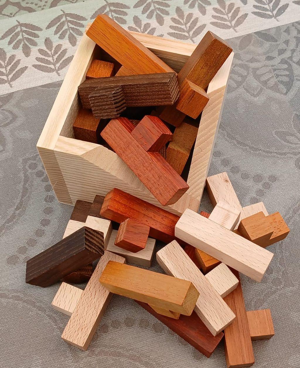
Its principle is fairly simple: it's composed of 25 identical wooden pieces, and a 5x5x5 cubic box. To solve the puzzle, one needs to pack the pieces into a 5x5x5 cube, without holes nor chunks dangling out, so that it fits into the box.

Here's what a single piece looks like: it's a 4x1x1 trunk, with a 1x1x1 cubic notch poking out from one side:

The puzzle is easy enough to understand, and the fact that it's basically all composed of cubes hints at the discrete nature of the problem, suggesting that it would lend itself well to an algorithm search. Exactly how to model the situation may not be completely obvious, though. We'll start setting the scene by modeling space itself, then we'll talk about individual pieces, first in isolation, then in the context of the whole puzzle. Along the way, we will need a bit of math; I'll do my best to explain theoretical notions as we encounter them.

First Steps Modeling our Problem

Since we're dealing with things that all ultimately decompose into 1x1x1 cubes, we can think of space as a grid of voxels (the 3D equivalent to a pixel) with integer coordinates. Mathematically, a position in that space is a vector with three integer coordinates¹.

The linear library provides the V3 type constructor for vectors of three coordinates; the type of positions will thus be V3 Int.

Since the box has dimensions 5x5x5 voxels, we'll say it contains all voxels whose coordinates are of the form V3 x y z, where x, y and z range from 1 to 5.

Since all pieces are identical, we can get away with modeling just one "generic piece", with arbitrary position and orientation. Every other piece can then be recovered simply by moving this "blueprint" around. We'll pick the disposition such that the piece's trunk extends from coordinates (0, 0, 0) to (0, 0, 3), and its notch is located at (0, 1, 2). We model that generic piece by simply providing the list of coordinates of the voxels that compose it:

genericPiece :: [V3 Int]
genericPiece = [ V3 0 0 0, V3 0 0 1, V3 0 0 2, V3 0 0 3, V3 0 1 2 ]

Now let's tackle the hard part: describing the ways a piece can be arranged inside the box.

Mathematically, the ways that an object may be moved around in space can be described by specifying a rotation around the origin, and a translation. A 3D rotation around the origin can be encoded by a 3x3 matrix, and a translation, by a 3-component vector:

data Disposition = Disposition
  { rotation    :: M33 Int
  , translation :: V3 Int
  } deriving Show

Now, for a given disposition of a piece, we need a way to get the coordinates of the cubes that compose the piece. To do that, we just apply the rotation and the translation to each cube of the generic piece.

dispositionCoordinates :: Disposition -> [V3 Int]
dispositionCoordinates disposition = fmap applyTransform genericPiece
  where
  -- Note that we are applying the translation after the rotation. We could
  -- technically apply the the translation first, but I think it makes
  -- more intuitive sense to first choose our piece's orientation and then
  -- translate it. In the end, what matters is that we stick to our convention.
  applyTransform :: V3 Int -> V3 Int
  applyTransform vector =
    translation disposition + (rotation disposition !* vector)

Our Action Plan to Enumerate All Dispositions

The Disposition datatype is able to represent any possible disposition of a piece in the box. What we'll need to solve the puzzle is to enumerate all those dispositions, but if we try to do so, we'll run into two problems:

1. Not all values of type Disposition actually correspond to a valid disposition:
   • The rotation field is of type M33 Int, but not all M33 Int matrices correspond to rotations: some of them encode transforms that mirrors their input, others, to transforms that inflate it, and others do weirder stuff yet.
   • Even in cases where the rotation field actually encodes a rotation, the specific disposition encoded by a given Disposition might not fit in the box.
2. The Disposition datatype is infinite (ignoring technicalities): it has fields of type V3 Int and M33 Int, which both have Int coefficients, and Int is infinite. So even if we wanted to list all possible Dispositions, we couldn't.

Fortunately, it turns out that there are only finitely many possible dispositions, so there's still hope that we might be able to list them all. Directly enumerating them would be too difficult, though, so we will decompose the task:

1. First, we'll make up a list of candidate dispositions. This list will have two important properties:
   • Any valid disposition will appear in the list, even though the list might still (and will) feature invalid ones.
   • The list will be finite, so we'll be able to enumerate it.
2. Then we'll define a predicate on dispositions, that is, a function of type Disposition -> Bool, which will tell us — this time with certainty — whether a given disposition is valid.

To get the full, exclusive list of valid dispositions, we'll then just need to filter out invalid dispositions from the list of candidate ones.

Enumerating Candidate Dispositions

A Disposition has two fields; let's look at each of those in detail. First, the rotation field. rotations are encoded by a value of type M33 Int. As we saw earlier, though, not all values of that type encode a rotation. Is there a simple way to narrow M33 Int down to an easily enumerated collection? There is!

To do that, we first need to talk a bit about what the coefficients of a 3x3 matrix represent. Say you have a 3D linear transform, and you want to write down the matrix M that corresponds to it (in the standard coordinate system with axes X, Y and Z). The first thing you do is apply the transform to the X axis. You end up with a vector that is no longer necessarily aligned with the X axis; instead, it has components along the X, Y and Z axis. The coefficients on the first row of the M correspond to how much of each of the three axes appear in our transformed X axis. Then the second row correspond to the same, but starting with the Y axis, and the third row, to the Z axis.

That's for a general linear transform. But we're dealing with the much more specific case of rotations in a voxel world. If you think a bit about what happens in you rotate one of the three axes when you rotate it in that context, you'll find that it either:

• Remains unchanged.
• Gets flipped.
• Turns into another axis.
• Turns into the flipped version of another axis.

In all four cases, the corresponding matrix row will contain a 1 or a -1 coefficient for the resulting axis, and a 0 coefficient elsewhere. This means that if we enumerate all possible matrices with coefficients -1, 0 and 1, we'll get all valid rotation matrices! We do so using Haskell's handy syntactic sugar for list comprehension:

candidateRotations :: [M33 Int]
candidateRotations = [
  -- The `M33` type is actually just two nested `V3` in a trench coat:
  V3 (V3 m11 m12 m13)
     (V3 m21 m22 m23)
     (V3 m31 m32 m33)
  | m11 <- [-1..1], m12 <- [-1..1], m13 <- [-1..1]
  , m21 <- [-1..1], m22 <- [-1..1], m23 <- [-1..1]
  , m31 <- [-1..1], m32 <- [-1..1], m33 <- [-1..1]
  ]

Again, keep in mind that this list contains many matrices that do not correspond to valid rotations. But all valid rotations do appear in it.

Now we'll need to narrow the possible translations down into a finite list too. The following paragraph is my attempt at explaining somewhat rigorously how we do that; it's a little convoluted, but the general idea is fairly intuitive: we care only about dispositions that fit in the box, so we can rule out any disposition that translates the genericPiece too far away.

Ok, now here's the "rigorous" explanation: the V3 Int type is able to encode arbitrarily long translations, but we're only interested in those that keep the piece in our 5x5x5 box. Taking a look at the genericPiece above, remark that it contains the cube at the origin, V3 0 0 0. Regardless of the rotation matrix we apply, it will leave that cube unchanged. This means that only the translation field impacts the origin cube. In other words, in any piece given by a value of type Disposition, the coordinates of the cube corresponding to the genericPiece's cube at the origin are exactly the translation's field coordinates. Since we want all the cubes in our piece to fit in the box, all coefficients must be between 1 and 5. So we can rule out any disposition whose translation field features coefficients outside that range, and we can finitely enumerate a list of candidate translations:

candidateTranslations :: [V3 Int]
candidateTranslations = [ V3 x y z | x <- [1..5], y <- [1..5], z <- [1..5] ]

Now that we have an enumeration of candidates for each of Disposition's fields, we can put them together to get a list of candidate Dispositions:

candidateDispositions :: [Disposition]
candidateDispositions =
  [ Disposition rot trans | rot   <- candidateRotations
                          , trans <- candidateTranslations ]

Filtering Out Remaining Invalid Dispositions

Now on to filtering out the remaining invalid dispositions! First we'll weed out invalid rotations. We don't need to get into the details here, but it turns out there's an easy way to tell whether a given 3x3 matrix encodes a rotation: a 3x3 matrix M encodes a rotation exactly when it is part both of the orthogonal linear group and the special linear group. In more concrete terms, this means M fulfils the following two conditions:

1. M multiplied by its transpose is the identity matrix.
2. M's determinant is 1.

In Haskell, this translates to:

-- | Does the given matrix encode a rotation?
isRotation :: M33 Int -> Bool
isRotation matrix = ((transpose matrix !*! matrix) == identity) &&
                    (det33 matrix == 1)

We're almost done describing all possible dispositions! We know what a valid rotation looks like, now the one problem we might still have is a piece arranged in such a way that it doesn't fit in the box. That's easy, we just need to check that each cube of the piece fits in the box:

pieceFitsTheBox :: Disposition -> Bool
pieceFitsTheBox disposition =
  all cubeFitsTheBox (dispositionCoordinates disposition)
  where cubeFitsTheBox :: V3 Int -> Bool
        cubeFitsTheBox (V3 x y z) = x >= 1 && x <= 5 &&
                                    y >= 1 && y <= 5 &&
                                    z >= 1 && z <= 5

And a valid disposition is one whose rotation field is actually a rotation, and which results in a piece that fits in the box:

isValidDisposition :: Disposition -> Bool
isValidDisposition disposition = isRotation (rotation disposition) &&
                                 pieceFitsTheBox disposition

Putting it all together, we get a list of all valid dispositions by starting from the list of candidate dispositions and filtering out invalid ones:

allValidDispositions :: [Disposition]
allValidDispositions = filter isValidDisposition candidateDispositions

We're pretty much done for this first blog post, but I'd like to prepare for the next one with one last step: our Disposition datatype served us well, but all we will need now to solve the puzzle is the actual coordinates of the cubes that compose the pieces. So we'll convert it all to coordinates:

allValidPieces :: [[V3 Int]]
allValidPieces = fmap dispositionCoordinates allValidDispositions

Phew! That was a little tedious, but now everything's in place for next part, where we'll leverage Haskell's conciseness to actually solve the puzzle in a very elegant way. See you then!